How does a LLM work?

We will implement a model that is compatible with GPT-2. But before that, here are some explanations to understand how it works.

A generative LLM is simply a neural network that takes tokens as input (the number of inputs corresponds to the context size of the model). The network has as much outputs as the size of the vocabulary (the number of different possible tokens). The values indicate the probability for each of the tokens to be next one. The raw output (logits) is a vector of values ranging from -∞ to +∞. The softmax function allows us to turn this into probabilities. In between, there are a number of layers. We will detail how they work in this article.

Here’s what it looks like:

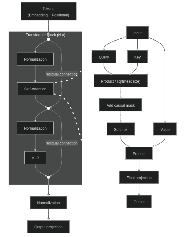
B̶̠̲̟̭̰͗̊̚͝ȇ̷̻̜̖͑̆̅̌̊ ̸̑̒̋͂͜n̵̦̮̼̞̲̘̅̋o̸̜̘͒̓t̴̫͒ ̶̹͉͋̀͊͘ȧ̴̠f̶̮͇͎͂̏̈̾ȑ̶͔̣̦̪a̸̭͎̓̈ḯ̵̬̙̱̫̤̾̽̈́͜d̴͉͓͇̠͒̄̊̌̈́. It's simpler than it sounds.

Note: You’re probably used seeing the diagram from the paper ”Attention is all you need” (Vaswani et al. 2017) which represents a encoder + decoder transformer. Here I represent the GPT-2 architecture described in the paper ”Language Models are Unsupervised Multitask Learners” (Radford et al. 2019) which is a decoder only (generative) transformer.

Prompt

We start with a text that we will place in the input of the model to generate the next token:

Hello, I’m a language model,

Tokenization (text to integers)

The text is then transformed into a series of tokens.

Hello	,	␣I	‘m	␣a	␣language	␣model	,
15496	11	314	1101	257	3303	2746	11

To achieve this transformation, a tokenizer is used. This example corresponds to the true values of the GPT-2 tokenizer. I won’t detail the creation of the tokenizer in this article to focus on how the neural network works.

Token Embeddings (integers to real vectors)

Then we project the token ids into the embedding space.

15496	11	314	1101	257	3303	2746	11
0.12	-0.05	0.33	-0.21	0.07	0.61	-0.30	0.00
-0.34	0.22	0.14	0.45	-0.18	-0.09	0.02	-0.07
0.56	-0.13	-0.27	0.02	0.39	0.18	0.47	0.09
0.03	0.40	0.58	-0.30	0.21	-0.42	0.11	-0.15
-0.11	0.01	-0.04	0.66	-0.50	0.25	-0.22	0.20
0.89	-0.29	0.10	-0.08	0.04	0.33	0.55	-0.02

To achieve this transformation, an embedding Pytorch module is used. It is simply a trainable dictionary. The size of embeddings is 6 so that the example remains understandable. In the GPT-2 model that we are going to implement, the size of the embeddings will be 1024. From now, unlike the previous step, I’ll use random values just for the example. These values depend on the training, and I have not trained a real model with an embeddings size of 6.

Position Embeddings

For each token position, its position vector is retrieved. The size of the vectors is the same as for the tokens embeddings.

pos0	pos1	pos2	pos3	pos4	pos5	pos6	pos7
0.05	-0.02	0.10	-0.07	0.03	0.06	-0.04	0.01
-0.01	0.08	-0.05	0.12	-0.09	0.02	0.07	-0.03
0.14	-0.06	0.04	0.09	-0.02	-0.08	0.11	0.00
-0.07	0.03	0.13	-0.10	0.05	0.01	-0.02	0.08
0.02	-0.04	0.06	0.00	0.09	-0.05	0.03	-0.01
0.09	0.01	-0.08	0.04	-0.03	0.10	-0.06	0.02

Here, an embedding Pytorch module is also used for this.

Final Embeddings (token + position)

We then add the two previous matrices.

15496	11	314	1101	257	3303	2746	11
0.17	-0.07	0.43	-0.28	0.10	0.67	-0.34	0.01
-0.35	0.30	0.09	0.57	-0.27	-0.07	0.09	-0.10
0.70	-0.19	-0.23	0.11	0.37	0.10	0.58	0.09
-0.04	0.43	0.71	-0.40	0.26	-0.41	0.09	-0.07
-0.09	-0.03	0.02	0.66	-0.41	0.20	-0.19	0.19
0.98	-0.28	0.02	-0.04	0.01	0.43	0.49	0.00

Now, our input is ready to move into the attention layers. Each input vector takes into account the token and its position.

If you have experience with using LLMs, it may seem strange to you to use an absolute position and combine it with the context tokens. For example, if you use a LLM as a chatbot, you will put the chat history in context up to a certain percentage. Next, you’re going to keep the end of the history, which will “slide” into the context. So it’s weird to use an absolute position vector to encode the position information of a given token, because this vector will change over time. As the history shifts in context, the model will not consider the relationships between tokens in the same way.

The GPT-2 positioning system also poses training problems. The context filling during inference must be similar to the size of the inputs in the training data, otherwise, the result will be a bit random.

This is probably the main flaw of the GPT-2 architecture. Today, LLMs use RoPE (Rotary Position Embedding) to replace absolute positioning. Instead of adding the positioning information in the input as in GPT-2, RoPE intervenes directly in the attention mechanism at the query and key levels, and allows to capture the relative relationships between tokens.

The system used by GPT-2 is simpler. This is why it is interesting to start there to learn how LLMs work. It’s a good introduction that will allow you to understand more complex architectures. But the use of absolute positioning is outdated for most uses.

Input normalization (transformer block)

Each layer begins with an input normalization. For each vector representing both a token and its position, we calculate the mean and standard deviation of its values (independently of the other vectors). Then apply the following formula to each value (x) of the vector:

y = bias + weight * (x - mean) / standard_deviation

As usual, weights and biases are obtained during the training. And actually, we don’t do this by hand, but use a LayerNorm module from Pytorch.

FYI, in more modern models, we use RMSNorm (root mean square normalization) which does not center on the mean and does not use bias. This method is a bit faster in terms of computation, and it works better for deeper networks.

Causal Self Attention (transformer block)

This is where the serious things begin!

We start by applying 3 linear transformations (weight * input + bias) to our input embeddings to get query, key and value matrices.

Query

15496	11	314	1101	257	3303	2746	11
0.12	-0.21	0.35	-0.15	0.05	0.62	-0.28	0.03
-0.30	0.25	0.14	0.48	-0.22	-0.05	0.07	-0.12
0.65	-0.12	-0.18	0.08	0.33	0.15	0.52	0.06
-0.02	0.39	0.67	-0.34	0.22	-0.36	0.06	-0.05
-0.07	-0.01	0.04	0.58	-0.36	0.17	-0.15	0.16
0.92	-0.24	0.05	-0.02	0.03	0.38	0.45	0.02

Key

15496	11	314	1101	257	3303	2746	11
0.18	-0.09	0.41	-0.26	0.11	0.68	-0.33	0.00
-0.36	0.31	0.08	0.55	-0.25	-0.09	0.10	-0.09
0.71	-0.21	-0.21	0.12	0.39	0.08	0.56	0.08
-0.05	0.45	0.69	-0.38	0.27	-0.43	0.11	-0.08
-0.10	-0.02	0.01	0.63	-0.39	0.22	-0.17	0.18
0.96	-0.30	0.00	-0.06	0.00	0.40	0.51	-0.01

Value

15496	11	314	1101	257	3303	2746	11
0.15	-0.18	0.38	-0.20	0.08	0.64	-0.31	0.02
-0.33	0.28	0.11	0.52	-0.24	-0.06	0.09	-0.11
0.68	-0.16	-0.20	0.10	0.36	0.12	0.55	0.07
-0.03	0.41	0.70	-0.36	0.24	-0.40	0.08	-0.06
-0.08	-0.02	0.03	0.61	-0.38	0.21	-0.18	0.17
0.95	-0.26	0.03	-0.03	0.02	0.41	0.48	0.01

Then we separate the attention heads. As the size of the embeddings chosen for this example is 6, we will say that we have 2 attention heads. For each head, the size of the embeddings is 3.

In the real case that we will implement, the size of the embeddings will be 1024 and we will have 16 attention heads. The size of a head will be 64.

Query (first head)

15496	11	314	1101	257	3303	2746	11
0.12	-0.21	0.35	-0.15	0.05	0.62	-0.28	0.03
-0.30	0.25	0.14	0.48	-0.22	-0.05	0.07	-0.12
0.65	-0.12	-0.18	0.08	0.33	0.15	0.52	0.06

Query (second head)

15496	11	314	1101	257	3303	2746	11
-0.02	0.39	0.67	-0.34	0.22	-0.36	0.06	-0.05
-0.07	-0.01	0.04	0.58	-0.36	0.17	-0.15	0.16
0.92	-0.24	0.05	-0.02	0.03	0.38	0.45	0.02

Key (first head)

15496	11	314	1101	257	3303	2746	11
0.18	-0.09	0.41	-0.26	0.11	0.68	-0.33	0.00
-0.36	0.31	0.08	0.55	-0.25	-0.09	0.10	-0.09
0.71	-0.21	-0.21	0.12	0.39	0.08	0.56	0.08

Key (second head)

15496	11	314	1101	257	3303	2746	11
-0.05	0.45	0.69	-0.38	0.27	-0.43	0.11	-0.08
-0.10	-0.02	0.01	0.63	-0.39	0.22	-0.17	0.18
0.96	-0.30	0.00	-0.06	0.00	0.40	0.51	-0.01

Value (first head)

15496	11	314	1101	257	3303	2746	11
0.15	-0.18	0.38	-0.20	0.08	0.64	-0.31	0.02
-0.33	0.28	0.11	0.52	-0.24	-0.06	0.09	-0.11
0.68	-0.16	-0.20	0.10	0.36	0.12	0.55	0.07

Value (second head)

15496	11	314	1101	257	3303	2746	11
-0.03	0.41	0.70	-0.36	0.24	-0.40	0.08	-0.06
-0.08	-0.02	0.03	0.61	-0.38	0.21	-0.18	0.17
0.95	-0.26	0.03	-0.03	0.02	0.41	0.48	0.01

This separation allows to make the calculations for each head independent. Thus, each head can pick up different relationships between the tokens, depending on the training of the model.

Now we’re going to focus on the first head. In practice, a dimension is added to the tensor and the calculation is carried out in parallel for all the heads.

We can now calculate the attention scores. To do this, we simply multiply the query matrix with the transpose of key (so that their dimensions are compatible). Then, the scores are divided by the square root of the size of the head to avoid the explosion of scores as the layers progress.

In the classical implementation of attention, the order of dimensions is reversed, sequence length and then head size. Here, for reasons of readability, I have used the opposite. So I first transposed the matrices and obtain this result for query * key / sqrt(head size).

	15496	11	314	1101	257	3303	2746	11
15496	0.3413	-0.1387	-0.0643	-0.0682	0.1973	0.0927	0.1700	0.0456
11	-0.1230	0.0702	-0.0236	0.1026	-0.0764	-0.1010	0.0156	-0.0185
314	-0.0665	0.0287	0.1111	-0.0206	-0.0385	0.1218	-0.1168	-0.0156
1101	-0.0826	0.0840	-0.0230	0.1805	-0.0608	-0.0801	0.0822	-0.0212
257	0.1862	-0.0820	-0.0383	-0.0545	0.1092	0.0463	0.0845	0.0267
3303	0.1363	-0.0594	0.1263	-0.0986	0.0804	0.2529	-0.0725	0.0095
2746	0.1695	-0.0360	-0.1261	0.1003	0.0892	-0.0895	0.2255	0.0204
11	0.0527	-0.0303	-0.0057	-0.0385	0.0327	0.0208	0.0068	0.0090

This matrix shows the relationship between each token. Since we want an auto-regressive model, each token should only see the previous tokens but not the following ones. For example, token 314 (I) is before token 1101 (‘m), so it should not have a relationship with it.

To do this, we use a triangular matrix that looks like this:

	15496	11	314	1101	257	3303	2746	11
15496	0	-∞	-∞	-∞	-∞	-∞	-∞	-∞
11	0	0	-∞	-∞	-∞	-∞	-∞	-∞
314	0	0	0	-∞	-∞	-∞	-∞	-∞
1101	0	0	0	0	-∞	-∞	-∞	-∞
257	0	0	0	0	0	-∞	-∞	-∞
3303	0	0	0	0	0	0	-∞	-∞
2746	0	0	0	0	0	0	0	-∞
11	0	0	0	0	0	0	0	0

We just add this matrix to the attention scores (with non-causal attention, for example in an encoder transformer, we wouldn’t do that). Then, we apply the softmax function to obtain probabilities. After the softmax function, the -∞ values will give a probability of 0.

	15496	11	314	1101	257	3303	2746	11
15496	1	0	0	0	0	0	0	0
11	0.4519	0.5481	0	0	0	0	0	0
314	0.3036	0.3339	0.3626	0	0	0	0	0
1101	0.2201	0.2600	0.2336	0.2863	0	0	0	0
257	0.2339	0.1789	0.1868	0.1838	0.2166	0	0	0
3303	0.1763	0.1450	0.1745	0.1394	0.1667	0.1981	0	0
2746	0.1602	0.1304	0.1192	0.1495	0.1478	0.1236	0.1694	0
11	0.1309	0.1205	0.1235	0.1195	0.1283	0.1268	0.1251	0.1253

Now that we have our matrix that indicates the degree of relationship between the tokens, we’re going to multiply it by the value matrix, which we haven’t used yet.

And here’s the result (actually, I transposed it back to a horizontal display like at the beginning).

15496	11	314	1101	257	3303	2746	11
0.1500	-0.0309	0.1232	0.0177	0.0544	0.1789	0.0544	0.0761
-0.3300	0.0044	0.0332	0.1747	0.0371	0.0222	0.0468	0.0253
0.6800	0.2196	0.0805	0.0900	0.1894	0.1595	0.2404	0.1960

Now you just have to reassemble the heads by concatenation to find the same shape as at the beginning. I did the math in my corner and here is the concatenated result.

15496	11	314	1101	257	3303	2746	11
0.1500	-0.0309	0.1232	0.0177	0.0544	0.1789	0.0544	0.0761
-0.3300	0.0044	0.0332	0.1747	0.0371	0.0222	0.0468	0.0253
0.6800	0.2196	0.0805	0.0900	0.1894	0.1595	0.2404	0.1960
-0.0300	0.2213	0.3917	0.1173	0.2208	0.0386	0.0867	0.0630
-0.0800	-0.0457	-0.0186	0.1818	0.0023	0.0826	0.0119	0.0538
0.9500	0.2589	0.1971	0.1632	0.1431	0.2351	0.2689	0.2020

All you have to do is apply one last linear transformation (the shape doesn’t change), and the attention mechanism is over for this block.

Attention residual connections (transformer block)

Here we add the input of the attention layer to the output. This technique allows to stabilize the training of deep networks, and among other things, to avoid the vanishing gradient problem.

Attention normalization (transformer block)

A normalization layer is applied again. This layer is different from the previous one (the one we applied to the input of the transformer block) only by its training (different weights and biases).

MLP (transformer block)

Finally, we pass the result through a classic MLP (multi layer perceptron). The first layer is a linear transformation whose output is 4 times the length of the embeddings. This operation allows the network to learn more complex relationships between the data during the training.

We then go through an activation function. In the context of GPT-2, this is GELU (Gaussian Error Linear Unit) but other functions are commonly used, for example SiLU (Sigmoid Linear Unit).

Finally, a last linear transformation brings the output back to the embedding size. This way, the data remains compatible with future attention layers.

MLP residual connections (transformer block)

Here we add the input of the MLP to the output.

Here’s the output of the transformer block (I’m going back to random values because I still haven’t trained a model with embeddings of 6).

15496	11	314	1101	257	3303	2746	11
0.0487	-0.0656	0.0198	-0.0476	0.0314	0.0831	0.0473	0.0298
-0.3558	0.0282	-0.1039	0.0416	-0.0845	-0.1447	-0.0559	-0.0896
0.1810	0.0717	0.0334	0.0180	0.0719	0.1013	0.0776	0.0626
0.0049	0.0706	0.0990	0.0542	0.0777	0.0069	0.0354	0.0214
0.0191	-0.0396	-0.0130	-0.0166	-0.0067	0.0174	-0.0001	0.0101
0.0634	0.0152	0.0798	0.0210	0.0512	0.1004	0.1036	0.0462

Final normalization

Once all the attention blocks have been passed, a final normalization is applied.

Output projection

Finally, we apply a last linear transformation to map from the embedding size to the vocabulary size. We then obtain output logits.

Sampling

The output of the network can be used to generate the next token. By applying the softmax function, we can transform the output into a vector indicating the probability of each token being the next.

You can then do greedy decoding, i.e. take the most likely token. But in practice, this is not used much because it gives boring and uncreative results.

You can simply randomly draw the next token based on probabilities.

It is also possible to divide the output vector by the temperature before applying the softmax function. A temperature greater than 1 will crush the probability gap and make the result more creative. Conversely, a temperature below one will amplify the differences and make the result more predictive.

Instead of directly drawing the token randomly according to probabilities, you can first limit the tokens by using top-p (you keep only the most likely tokens as long as the sum of their probability does not exceed p) and/or top-k (you keep only the k most likely tokens).

Text generation

To continue the text generation, simply place the new token at the end of the inputs and make a new pass in the network.

Don’t miss my upcoming posts — hit the follow button on my LinkedIn profile