Hello World neural networks (part 2)
Published on Feb 28, 2025 in AI Fundamentals
This is the continuation of this article.
In the previous article, you learned how to create an artificial neuron, or perceptron, and train it. This time, we’re going to create a real neural network.
There are many topologies of neural networks. For example, CNNs (Convolutional Neural Networks) which are used in computer vision, or RNNs (Recurrent Neural Networks) which are used for time series forecasting. There are also of course transformers that have become popular in recent years with ChatGPT, which are used for NLP (Natural Language Processing).
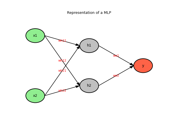
Here we will use an MLP or multi-layer perceptron. This is a special case of a feedforward network with an input layer, an output layer, one or more hidden layers in between. The outputs of each layer are connected to all the neurons of the next layer.
Unlike CNNs that allow a spatial relationship between the data or RNNs that allow a temporal relationship between the data, MLPs are used when there is no specific organization in the data.
This time, we will be teaching XOR to our network. To do this, we’re going to use a two-input network, a hidden layer with two neurons, and an output layer with one neuron.
For the training, we’re going to use backpropagation and gradient descent. The gradient descent is a general-purpose optimization algorithm that allows you to find the minimum of a function. Here, our goal is to minimize the loss function.
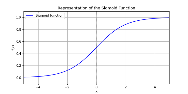
We’re going to use a sigmoid as an activation function (1 / (1 + exp(-x))), because for the gradient descent, we need the derivative and the Heaviside function is not differentiable at the origin.
What we’re going to do is actually quite similar to what we did in part 1. Except that we’re going to use the derivative of the activation function in the calculation of the delta that we’re going to apply to the weights to make them converge. And that we’re going to backpropagate the error, from the output layer to the hidden layer, to correct the weights.
Rather than overwhelming you with equations, I’m going to explain the logic that we’re going to use in simple words. I promised that this series of articles would be understandable with a teenager’s level of math. And we study partial derivatives at university. But you won’t need that to understand.
The result of the sigmoid function evolves between 0 and 1. This is good because in our case, we want a final result between 0 and 1.
The derivative of a function indicates its gradient at a given location. This is what the derivative of a sigmoid looks like.
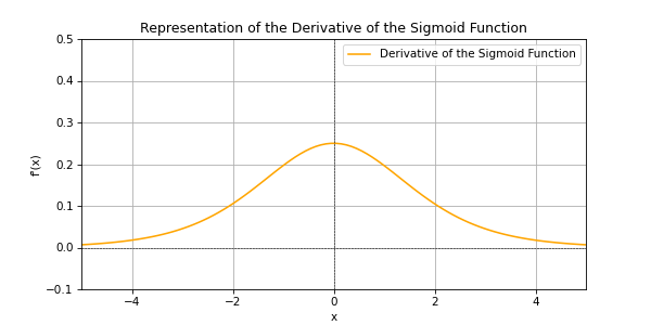
This means that when the result of the function is 0.5 (at the origin), the derivative is at its highest, and the weights will change faster than when the result of the function is close to 0 or 1. That’s a good thing because we want 0 or 1 and we’re not interested in an intermediate result. Now you understand the interest of using the sigmoid and its derivative.
Of course, nothing is perfect and this usage also causes problems. The further away from the origin, the lower the gradient. This causes what’s called the vanishing gradient problem. But our network is simple enough that this will not cause problems.
Here’s the full code to implement all of this.
import random
import math

class NeuronMLP:
    def __init__(self, n_inputs):
        # Random initialization of weights and bias
        self._weights = [random.uniform(-1, 1) for _ in range(n_inputs)]
        self._bias = random.uniform(-1, 1)

    def _activation_function(self, sum):
        # Sigmoid activation function
        return 1 / (1 + math.exp(-sum))

    def activation_derivative(self, output):
        # The derivative of the sigmoid is f'(x) = f(x) * (1 - f(x))
        # Here, f'(x) = output * (1 - output)
        # because we have already applied the sigmoid function to calculate the output
        return output * (1 - output)

    def calculate_output(self, inputs):
        # Calculate the dot product of inputs and weights and add bias
        # Then apply the activation function
        self._inputs = inputs
        sum = 0
        for i in range(len(inputs)):
            sum += inputs[i] * self._weights[i]
        sum += self._bias
        return self._activation_function(sum)

    def update(self, delta, learning_rate):
        # Update weights and bias
        for i in range(len(self._weights)):
            self._weights[i] += learning_rate * delta * self._inputs[i]
        self._bias += learning_rate * delta

class NetworkMLP:
    def __init__(self):
        # Initialize the layers of the network
        # 2 neurons in the hidden layer and 1 output neuron
        self._hidden_layer = [NeuronMLP(2) for _ in range(2)]
        self._output_neuron = NeuronMLP(2)

    def _forward_propagation(self, inputs):
        # Calculate the outputs of the hidden layer
        # and use the results as inputs for the output neuron
        # to calculate the final output
        hidden_outputs = [neuron.calculate_output(inputs) for neuron in self._hidden_layer]
        final_output = self._output_neuron.calculate_output(hidden_outputs)
        return final_output

    def _back_propagation(self, inputs, target_output, learning_rate):
        # Backpropagation algorithm
        # Perform the forward propagation
        final_output = self._forward_propagation(inputs)
        # Calculate the error and deltas for the output and hidden layers
        output_error = target_output - final_output
        output_delta = output_error * self._output_neuron.activation_derivative(final_output)
        hidden_deltas = []
        for i, neuron in enumerate(self._hidden_layer):
            hidden_delta = output_delta * self._output_neuron._weights[i] * neuron.activation_derivative(neuron.calculate_output(inputs))
            hidden_deltas.append(hidden_delta)
        # Update the weights and bias of the output and hidden neurons
        self._output_neuron.update(output_delta, learning_rate)
        for i, neuron in enumerate(self._hidden_layer):
            neuron.update(hidden_deltas[i], learning_rate)

    def train(self, input_vectors, output_vectors, learning_rate=0.1):
        # Train the network using backpropagation
        # Calculate the total loss for all input vectors
        # Return the average loss
        total_loss = 0
        for i in range(len(input_vectors)):
            self._back_propagation(input_vectors[i], output_vectors[i], learning_rate)
            prediction = self._forward_propagation(input_vectors[i])
            total_loss += (output_vectors[i] - prediction) ** 2
        return total_loss / len(input_vectors)

    def calculate_output(self, inputs):
        # Calculate the output of the network for a given input (round the output to 0 or 1)
        return round(self._forward_propagation(inputs))

# Define the input vectors and output vectors
input_vectors = [[0, 0], [0, 1], [1, 0], [1, 1]]
output_vectors = [0, 1, 1, 0]

# Create a neural network
network = NetworkMLP()

# Train the network
learning_rate = 0.1
max_epochs = 1000000
for i in range(max_epochs):
    loss = network.train(input_vectors, output_vectors, learning_rate)
    if (i+1) % 1000 == 0:
        print(f"Epoch {i+1}: Loss = {loss}")
    if loss < 0.0001:
        break

# Test the network
for inputs in input_vectors:
    output = network.calculate_output(inputs)
    print(f"Input: {inputs}, Output: {output}")
From this code, it can be fun to play around with the settings to see what happens.
For example, increase the learning rate with steps of 0.1 and observe the result. Then restart the program several times. You will find that sometimes the training will be much faster. But the more you increase the learning rate, the more likely the network is to never converge.
You can also change the loss threshold from 0.0001 to 0.001 for example. It will also reduce the learning time, but sometimes the network will not have had time to converge and will give bad results.
Beyond technique and mathematics, training an AI model requires a certain amount of empirical know-how. You can start learning this now.
If you read the research papers to find out why one option is used over another, you will find that often, many tests have been done, followed by statistics, which show which is the best option in given circumstances.
When you want to train a model with a large dataset, it is always important to test on a small extract of the data to see how the network behaves with this data.
Don’t miss my upcoming posts — hit the follow button on my LinkedIn profile