From overfitting to explainability, how to train a neural network

In a previous article I discussed in a theoretical way the training of neural networks, and the concepts of underfitting and overfitting.

In this article, you will discover how it works in concrete terms. To do this, we will train a classification model.

In my “AI Fundamentals” section, I have so far discussed the creation of neural networks that learn the behavior of logic gates. This context is very special because there are only four possible inputs. So we used all of them to train our model. We didn’t have any problems with generalization, since our model saw all the possible data during its training.

In a real case, you have to separate the dataset in two. One part for training and another for evaluation. The goal of the training is to minimize the error of the expected output (training loss), but also to check the model’s ability to generalize by evaluating its predictions on data that the model has never seen (evaluation loss).

The scikit-learn library provides functions for creating datasets with certain statistical properties. This is very handy for experimentation and we will use it to create a classification dataset. At the end of this article, I’d like to touch on the topic of explainability, and you’ll see that I have a particular interest in using a synthetic dataset rather than real data.

We will create a binary classification dataset with ten features, five of which are informative. To make this example less abstract, the ten features could be information about people. Our classes could be “has heart disease” or “has no heart disease.” Blood pressure or cholesterol levels could be informative features (correlated with the result of the classification) while eye color or level of education would be non-informative features.

Here’s the code we’re going to use. If you have followed my previous articles in “AI Fundamentals”, nothing very complicated here.

import matplotlib.pyplot as plt
from sklearn.datasets import make_classification
import torch
import torch.nn as nn
import torch.optim as optim
from torch.utils.data import DataLoader, TensorDataset, random_split

# Generate synthetic data for binary classification
X, y = make_classification(n_samples=1000, n_features=10, n_informative=5, n_redundant=0, n_classes=2, random_state=42)
# Convert to PyTorch tensors
data = torch.tensor(X, dtype=torch.float32)
labels = torch.tensor(y, dtype=torch.long)
# Create a dataset and split into training and validation sets
dataset = TensorDataset(data, labels)
train_size = int(0.8 * len(dataset))
val_size = len(dataset) - train_size
train_dataset, val_dataset = random_split(dataset, [train_size, val_size])
# Create data loaders with batch size 32
# When using a batch, the model updates its weights based on the average loss of the batch
# This helps to stabilize the training process and can lead to better generalization
# Shuffling the training data helps to ensure that the model does not learn any spurious patterns
# in the order of the data
train_loader = DataLoader(train_dataset, batch_size=32, shuffle=True)
val_loader = DataLoader(val_dataset, batch_size=32, shuffle=False)
# The first layer maps the input features to a hidden layer with 50 neurons
# This allows the model to learn more complex patterns in the data
# The GELU activation function is a smooth approximation of the ReLU function
# The second layer maps the hidden layer to the output layer with 2 neurons (for binary classification)
# The model uses the default PyTorch random weights
model = nn.Sequential(
    nn.Linear(10, 50),
    nn.GELU(),
    nn.Linear(50, 2)
)
# Cross-entropy loss is a common loss function for classification tasks
criterion = nn.CrossEntropyLoss()
# Adaptive Moment Estimation (Adam) is also a popular optimization algorithm
optimizer = optim.Adam(model.parameters(), lr=0.001)

train_losses = []
val_losses = []
for epoch in range(1000):
    model.train()
    epoch_train_loss = 0.0
    for batch_data, batch_labels in train_loader:
        optimizer.zero_grad()
        outputs = model(batch_data)
        loss = criterion(outputs, batch_labels)
        loss.backward()
        optimizer.step()
        epoch_train_loss += loss.item()
    avg_train_loss = epoch_train_loss / len(train_loader)
    train_losses.append(avg_train_loss)
    model.eval()
    epoch_val_loss = 0.0
    with torch.no_grad():
        for val_data, val_labels in val_loader:
            val_outputs = model(val_data)
            val_loss = criterion(val_outputs, val_labels)
            epoch_val_loss += val_loss.item()
    avg_val_loss = epoch_val_loss / len(val_loader)
    val_losses.append(avg_val_loss)
    print(f'Epoch {epoch+1}, Training Loss: {avg_train_loss}, Validation Loss: {avg_val_loss}')
    if avg_train_loss < 0.01:
        break

plt.figure(figsize=(10, 5))
plt.plot(train_losses, label='Training Loss')
plt.plot(val_losses, label='Validation Loss')
plt.xlabel('Epochs')
plt.ylabel('Loss')
plt.title('Training and Validation Loss')
plt.legend()
plt.savefig('training.png', dpi=75)
plt.show()

I’ve set a seed for the dataset, so every time you run the program, you’ll have the same data. On the other hand, I didn’t put a seed for PyTorch and the initialization of the weights will be different for each training.

We run the program and here is the result.

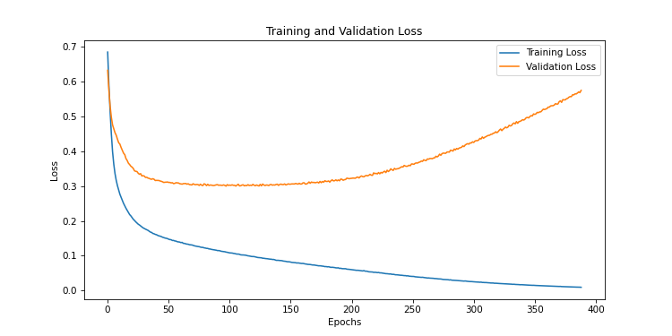
We realize that as the epochs progress, the model is more and more accurate on the training data. But these predictions are less and less correct on the evaluation data. This is a typical case of overfitting. The model has stored the data but is unable to generalize.

To fix this, we’re going to add a dropout layer to our model. This layer will be active during the training phase, initiated by model.train(), but not during inference phase, initiated by model.eval(). We will define a probability p and each neuron will be randomly deactivated, according to this probability. Outputs will be multiplied by 1/(1-p) to maintain the scale of activations.

Let’s start with a probability of 0.5

model = nn.Sequential(
    nn.Linear(10, 50),
    nn.GELU(),
    nn.Dropout(0.5),
    nn.Linear(50, 2)
)

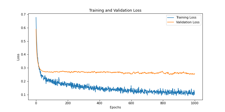
We notice that the validation curve does not diverge as in the previous training. But we still have an overfitting problem, because the curve is too high compared to the training loss.

Let’s try with a probability of 0.9

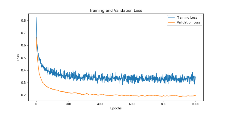
This time, the evaluation curve is below the training loss curve. The dropout rate is too high, and the model has trouble learning the relationships between the data. This is a typical case of underfitting.

Let’s try an intermediate value like 0.7

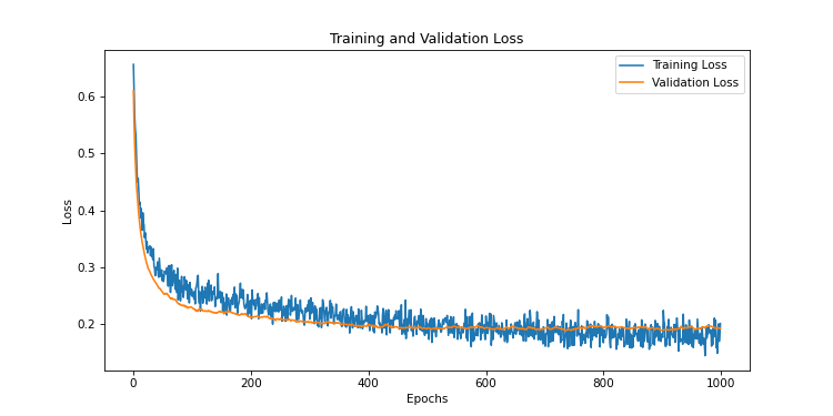
This time, it’s good! The training and evaluation curves are close, the evaluation very slightly above. That’s exactly what we want. Our model is therefore well trained. Since the initialization of weights is not fixed by a seed, it is possible that this value does not always work for a well-trained model. There is always a part of RNG in the training of a model.

Now let’s talk about the explainability of neural networks. It is common to hear that neural networks are black boxes and that we do not really understand what they do. In reality, it is possible to analyze them and understand how they work. They can even tell us things about the nature of our data.

We have a hidden layer with 50 neurons and ten inputs. Each feature is therefore associated with 50 weights. Add this code to the end of the program. This will draw blue bars ranging from zero to the weight mean for each feature, with a visualization of the standard deviation.

weights = model[0].weight.data.numpy()
plt.figure(figsize=(10, 6))
plt.bar(range(weights.shape[1]), weights.mean(axis=0), yerr=weights.std(axis=0), capsize=5)
plt.xlabel('Features')
plt.ylabel('Average Weights')
plt.title('Weight of the Input Layer')
plt.xticks(range(weights.shape[1]), [f'Feature {i+1}' for i in range(weights.shape[1])])
plt.savefig('weights.png', dpi=75)
plt.show()

Here is the result.

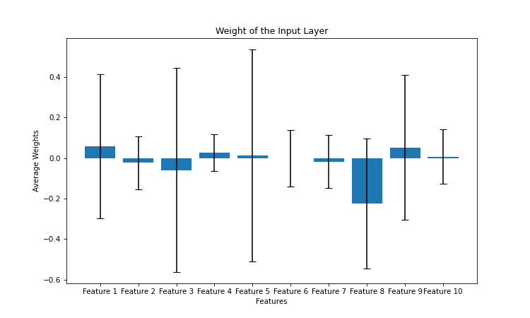
We notice that for features 2, 4, 6, 7 and 10, the average weight is close to zero and the standard deviation is small. This means that these features do not take part in the classification. These are of course the five non-informative features that we defined when creating our synthetic dataset.

The way the network works is explainable, and if we had worked on real data, we could have deduced which features are really correlated with the result of the classification, and which features are not, simply by analysing the weight of the network.

Don’t miss my upcoming posts — hit the follow button on my LinkedIn profile