Hello World neural networks (part 1)

In recent years, there has been a lot of talk about AI. But even for technical people, it remains quite esoteric.

With machine learning, we don’t implement logic. The system learns it from the data.

This may surprise you, but it’s basically very simple to create a neural network and train it.

You may think that you have to be a math genius. But any teenager has the necessary basics in mathematics to understand the example that I’m going to share with you.

I think that as in many areas, there is a lot of gatekeeping, conscious or not. Here, my goal is to share tutorials without unexplained jargon, accessible to all.

To understand this example, you will need to know a minimum of Python. In order to fully understand how this works, we will create a neural network from scratch without any specialized libraries. No numpy or pytorch this time.

Well, actually, I lied. For this first example, we are not going to create a neural network, but a single neuron.

In part 2, we will create a real neural network. But before that, you will see that we can already teach a few things to a single neuron.

In our case, we are going to train our neuron to behave like an OR logic gate. I know, it’s not very sexy. But this is the Hello World of neural networks.

Before we move on to practice, we need just a little theory. Nothing very complicated, don’t worry.

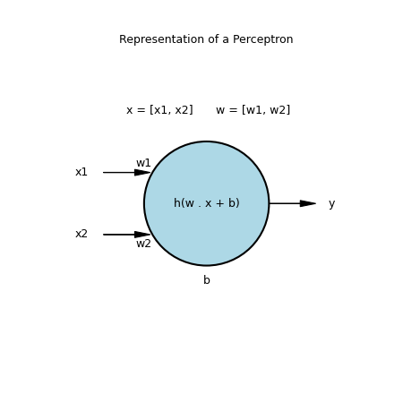
An artificial neuron, also called a perceptron, is a mathematical function which is inspired by the functioning of a real neuron (with inputs, an activation condition, and an output). In our case, the function we are going to use is:

f(x) = h(w . x + b)

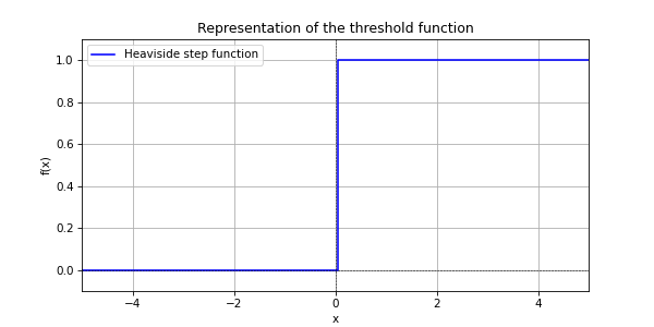
h is the Heaviside step function

w is a weight vector

x our input vector

b is the bias

So we have a neuron with n inputs (in our case, our neuron will have 2 inputs) and one output.

Each input has a weight, initially chosen randomly. With training, we will make these weights evolve so that the neuron gives the expected result.

The input values and the weights constitute the vector x and w.

To calculate the output (the result of the function), we start by doing the dot product of the input vector with the weight vector. With two dimensions it is simply w1 × x1 + w2 × x2.

Then we add the bias. Bias does not depend on inputs and it allows us to shift the origin, to avoid that for a zero input vector, the output is necessarily zero, which would limit the learning possibilities of our neuron.

Then we apply the step function. If the result is negative, the neuron’s output is 0, otherwise it is 1.

Now let’s implement this in Python.

import random

class Neuron:
    def __init__(self):
        # Random initialization of weights and bias
        self._weights = [random.random(), random.random()]
        self._bias = random.random()

    def _activation_function(self, sum):
        # Threshold activation function
        if sum >= 0:
            return 1
        else:
            return 0

    def calculate_output(self, inputs):
        # Calculate the dot product of inputs and weights and add bias
        # Then apply the activation function
        sum = 0
        for i in range(len(inputs)):
            sum += inputs[i] * self._weights[i]
        sum += self._bias
        return self._activation_function(sum)

Now that we have our neuron, we have to train it. As it stands, it has random weights and bias. It will give random results.

To train it, we will use training vectors. In our case, it is simply the truth table of an OR logic gate.

We call “epoch” the fact of applying all the training data once. For each epoch, we will apply each input vector and calculate the output according to the weights and the current bias. Then calculate the error between our prediction and the expected result. And then we will correct the weights and bias according to the error and the learning rate that we have defined.

The learning rate is a factor that prevents the weights from changing too quickly, which can lead to chaos and prevent the network from converging towards the expected result. The value used is usually between 1e-1 (0.1) and 1e-5 (0.00001).

It is also possible to use a decreasing rate as a function of epoch or an evolutionary rate as a function of gradient (how quickly the model converges). But in our case, we’re just going to use 0.1.

We will also measure the loss. The loss allows us to quantify the difference between our predictions and the expected results.

To do this, we will use the mean square error (MSE). Another complex expression to express something simple. It is simply the sum of the squared errors for each prediction, divided by the number of training vectors to obtain an average value.

The goal of training is to minimize loss. In general, the goal of training is to reach a small value, for example 1e-6. In our case, since we are not using continuous values but discrete values (zero or one), we will consider the training to be over when the loss is zero.

Let’s implement all of this in Python and you’ll see that it’s much simpler than it sounds:

import random

class Neuron:
    def __init__(self):
        # Random initialization of weights and bias
        self._weights = [random.random(), random.random()]
        self._bias = random.random()

    def _activation_function(self, sum):
        # Threshold activation function
        if sum >= 0:
            return 1
        else:
            return 0

    def calculate_output(self, inputs):
        # Calculate the dot product of inputs and weights and add bias
        # Then apply the activation function
        sum = 0
        for i in range(len(inputs)):
            sum += inputs[i] * self._weights[i]
        sum += self._bias
        return self._activation_function(sum)

    def _calculate_loss(self, input_vectors, targets):
        # Calculating the Mean Square Error
        total_loss = 0
        for i in range(len(input_vectors)):
            prediction = self.calculate_output(input_vectors[i])
            total_loss += (targets[i] - prediction) ** 2
        return total_loss / len(input_vectors)

    def train(self, input_vectors, targets, learning_rate):
        # Training the neuron using the Perceptron Learning Algorithm
        for i in range(len(input_vectors)):
            prediction = self.calculate_output(input_vectors[i])
            error = targets[i] - prediction
            for j in range(len(self._weights)):
                self._weights[j] += learning_rate * error * input_vectors[i][j]
            self._bias += learning_rate * error
        return self._calculate_loss(input_vectors, targets)

    def __str__(self):
        return f"Weights: {self._weights}\nBias: {self._bias}"

# Define the input vectors and targets
input_vectors = [[0, 0], [0, 1], [1, 0], [1, 1]]
targets = [0, 1, 1, 1]

# Create a neuron
neuron = Neuron()

# Train the neuron
learning_rate = 0.1
max_epochs = 100
for i in range(max_epochs):
    loss = neuron.train(input_vectors, targets, learning_rate)
    print(f"Epoch {i+1}: Loss = {loss}")
    if loss == 0:
        break

# Test the neuron
print(f"\nTrained neuron\n{neuron}")
print("\nPredictions for input vectors")
for input_vector in input_vectors:
    prediction = neuron.calculate_output(input_vector)
    print(f"Input: {input_vector}, Prediction: {prediction}")

By running this program, you will find that in a few epochs, the neuron will converge and give the expected results.

If you restart the program several times, as the starting point is random, the neuron will converge more or less quickly.

You may decide to teach your neuron something else, such as how to behave like an AND logic gate. To do this, simply change the line that defines the targets variable.

targets = [0, 0, 0, 1]

With this new training data, your neuron will become an AND gate at the end of its training.

We will now test the limits of what this simple neuron can learn. Replace the targets variable with the results of an XOR gate.

targets = [0, 1, 1, 0]

When you restart the program, you will find that the neuron will not converge and even after 100 epochs, it will still not give the correct results.

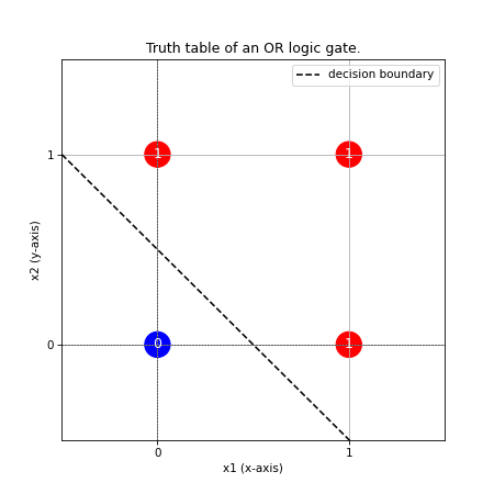
You’re probably wondering why XOR is different. It’s a question of linear separability. A simple neuron can only learn a function that is linearly separable. This means that if we plot our truth table in a plane (x1 for the x-axis and x2 for the y-axis), we can separate the zeros and ones by a straight line (or a hyperplane for n dimensions).

Here is for example of the truth table of the OR.

Now, if we plot the truth table for XOR, we realize that zeros and ones are not linearly separable.

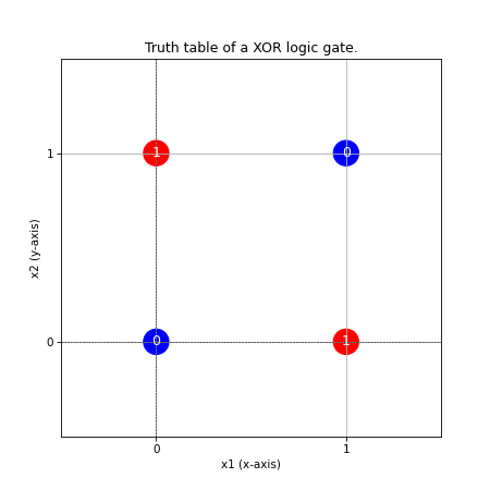
To learn XOR, we need a multi-layered neural network (multi-layer perceptron or MLP). This type of network is capable of creating nonlinear decision boundaries.

This will be the subject of part 2 of this article. To train such a model, we will use backpropagation and gradient descent. You’ll see that it’s not that much more complicated than what we’ve just done.